
Hop depth, reliability, relay capacity and segmented architecture
Abstract
Linear wireless mesh networks are attractive for perimeter monitoring, pipelines and distributed infrastructure, yet line length is not equivalent to a single radio link length. This article studies the 1 –100 km linear cases analyzed in MESH2026 using explicit hop spacing and gateway placement assumptions. A reference 100 m hop gives 500 hops over 50 km and exceeds the current source firmware layer encoding, while a segmented architecture reduces operational exposure. A simplified independent link model demonstrates the sensitivity of long chains to per hop delivery quality and retransmission limits. Calculated delay estimates illustrate why scheduling and gateway sectorization must be designed before deployment. The results are analytical and require field confirmation.
Keywords: wireless mesh networks; sensor networks; linear mesh 1 to 100 km; analytical modeling; reliability; network design.
1 Introduction
Wireless mesh designs connect nodes using multiple wireless links and forwarding relays, but the existence of an alternate link does not by itself guarantee end to end service. Performance depends on radio quality, control traffic, source reporting rates, topology changes and gateway capacity. This study addresses one distinct subset of those coupled design concerns, using the models and engineering constraints developed in MESH2026-v07. Its findings are analytical statements with explicit assumptions rather than claims about a completed controlled deployment.
The objective is to define a technically traceable decision framework that converts the supplied study into testable engineering criteria. The manuscript draws solely on the source report and bibliographic entries present in that report. References retain the original source numbering so each item can be reconciled directly with the underlying bibliography. No new externally obtained sources are introduced.
2 Analytical Scope and Method
The method proceeds by identifying the system boundary, selecting a small number of measurable state variables, deriving a simplified relationship or comparison, and then distinguishing mathematical consequences from assumptions that require experimental verification. Conceptual drawings show component or information relationships; calculated charts visualize nominal conditions. They are not field measurements. This separation is especially important in wireless systems, where terrain, interference, retransmission policy and time synchronization can dominate apparent theoretical advantage.
Source basis: MESH2026-v07, sections 4.2, 4.2.1, 4.2.2, 4.2.3. Reference numbers preserve the numbering of its chapter 7 bibliography. The analytical figures are original illustrations of stated assumptions, not experimental observations.

Figure 1. Functional architecture developed from the relevant MESH2026 concepts; schematic, not a tested implementation.
3 Linear topology is a special network case
A line geometry has little path diversity compared with a two dimensional mesh, because there are relatively few alternate neighbors around a failed relay. A gateway positioned at one end of the line receives the accumulated reports from all downstream sensors. In such a system the first relay can become a capacity, battery and single point of failure bottleneck. Mesh self healing must not be presumed when the line lacks physical redundant links.
The source study compares nominal line lengths of 1, 5, 10, 25, 50 and 100 km. With 100 m spacing, these correspond to 10, 50, 100, 250, 500 and 1000 hops, respectively. Those counts are geometric planning values only. Real effective hop spacing depends on path loss, vegetation, antenna height, interference and the packet delivery target. The design must also distinguish sensor spacing from relay spacing because a sensor can be farther from the next relay than expected from a regular map. [6], [77].
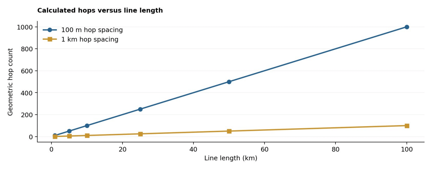
Figure 2. Calculated or qualitative illustration of the design mechanism. Axes and assumptions are described in the main text.
4 Firmware topology limits
The reference implementation discussed in MESH2026 stores meshLayer in a 7 bit field: values 0 to 127, with 127 reserved for unknown or recovering topology. About 126 operative layers therefore fit safely without changing the representation. A 500 hop system cannot be declared deployable by choosing 100 m antennas if the application cannot encode or correctly schedule those layers. Changing the field width entails auditing advertisements, persistence, time offsets, diagnostic software and backward compatibility.
A sector based design creates shorter independent lines with their own gateways or collection points. For a 50 km site with 100 m hop spacing, partitioning into manageable segments can reduce maximum route length and reduce the number of forwarded packets passing through a single first relay. It also changes infrastructure requirements, connectivity between gateways and protection of the wider backhaul. Such tradeoffs should be explicit in the deployment budget. [20], [29].
Table 1. Scope of the principal design comparison.
Line length Hops at 100 m Ideal delay at 120 s/hop One hour per hop
1 km 10 20 min 10 h
5 km 50 1 h 40 min 50 h
10 km 100 3 h 20 min 100 h
25 km 250 8 h 20 min 250 h
50 km 500 16 h 40 min 500 h
100 km 1000 33 h 20 min 1000 h
5 Reliability under repeated hops
For independent per attempt success p, an idealized link with up to r attempts has success peff = 1 − (1 − p)^r. The chain probability under identical independent effective links is Pend = peff^h. This approximation ignores correlated errors, queue overflow and retransmission scheduling, but exposes the strict per hop requirement of a long chain. For 500 hops and three attempts, p = 0.95 yields about 93.9% calculated end to end success, while a modest decrease in p can produce a much larger loss.
Physical failures invalidate independent probability assumptions. A storm, common interference source, damaged antenna set or synchronized timeslot collision can affect many adjacent links together. Consequently, packet success estimates must be paired with real multi hour traces, controlled outage tests and measurements of route recovery. A network that achieves strong delivery at rest may be unsuitable if every gateway report arrives hours after its useful decision window. [2], [78].
6 Latency, timing and traffic concentration
A useful bounding calculation is D ≈ h·Tslot for a pipelined schedule in which the next relay is ready each successive slot. A duty cycle plan that provides only one useful forwarding opportunity per hour can instead produce a delay approaching h hours. In the source comparison, an ideal 120 s progression over 500 hops corresponds to 16 h 40 min, whereas one hop per hour gives 20.83 days. These are scheduling scenarios, not measured field latencies.
The first hop near a terminal gateway must handle reports created by all nodes in the upstream segment. Payload aggregation and reporting interval must therefore be checked against the actual medium access budget and collision rate. A small number of raw payload bytes does not imply adequate throughput because beacons, route discovery, acknowledgements, channel contention and failed attempts consume air time as well. [70], [71].
Evaluation parameters
A reproducible trial should log per-node packet identifiers, generation and reception timestamps, route changes, radio retransmissions, queue age and battery current. All measurement and reporting intervals, payload formats, antenna geometry and firmware revisions should be recorded. Reliability must be reported with variation over trials, not as a single best-run percentage. A successful link in one season or installation position is not equivalent to a verified network-level service guarantee.
7 Experiment and applicability limits
A credible demonstration should instrument all hops, maintain synchronized timestamps, and test nominal operation and multiple failure positions. Record join time, farthest node delivery, packet age, longest route, firmware layer encoding and measured current draw of gateway-adjacent relays. The final design should classify each planned segment by service requirements, not only geographic distance.
The line examples do not establish a universal maximum mesh length. They establish conditions that a proposed design must satisfy. Results are especially sensitive to environmental loss, required packet freshness, sector gateway availability and radio schedule. The analysis supports multi gateway sectorization as a prudent candidate for long line service, pending field validation. [2].
8 Reproducible Experiment Design
Sector length and hop count trial
Test increasing chains with one gateway, then introduce a second collection point while holding total reporting load constant. Force failure of the first and central relays in separate trials. Verify layer encoding before the longest chain is attempted. Synchronize send and receive clocks to distinguish radio transfer delay from waiting for communication windows.
All trials should state the hypothesis before measurements begin. In particular, baseline and modified networks must generate a comparable number of application messages under identical payload semantics. Time synchronization, radio configuration, antenna placement and test duration should be documented. Apply a predefined definition of a valid delivery, including how duplicate frames, acknowledgements, partial packets and expired records are treated. Report distributions and uncertainty rather than interpreting isolated examples as population-level network behavior.
The primary measurement vector is: Maximum encoded layer, far-node delivery, queue age, link retries, convergence time and critical relay current. The experiment should archive raw records and configuration files so that independent reviewers can reconstruct packet success, route depth and energy exposure. Failed configurations and unavailable nodes must remain in the results table rather than being discarded as outliers. Where an event is delayed by buffering, store both the origin timestamp and the gateway arrival timestamp to avoid falsely classifying a stale packet as timely delivery.
9 Model Sensitivity and Acceptance Criteria
A design parameter has operational meaning only relative to an application threshold. For packet delivery, an acceptable loss ratio may differ between a periodic weather reading and an emergency alarm. For latency, a median value can be misleading when occasional extreme delay is harmful. Therefore the acceptance plan should name the threshold and its aggregation level: individual node, gateway sector or whole deployment. At minimum, retain a reliability target, a maximum age for useful data, and a minimum expected autonomy for each energy role.
Sensitivity analysis should vary one major assumption at a time and then test coupled effects. Candidate variables include per-hop reception probability, reporting frequency, number of downstream children, active listening duration, gateway count and available battery capacity. An improvement observed under one parameter combination may disappear when the network is congested or when temperature reduces battery availability. The purpose of a sensitivity plot is to identify which physical measurement would most change the final design decision, not to predict field performance without evidence.
The product model of hop probabilities is appropriate only for a stated independence assumption; correlated failures require repeated end-to-end observation.
A final acceptance matrix should include four outcomes: the test condition, the expected service limit, the observed numerical result and the engineering decision. The source technical study supports the selection of variables and design mechanisms, but a numerical pass/fail result requires an actual implemented protocol and controlled measurements. The distinction prevents a model assumption from being silently promoted to verified specification.
Evaluation scenario matrix
Scenario Variable held constant Question to resolve
Same radio / payload / gateway Does the reference service meet its Nominal baseline position target?
Same node count and physical Does age or packet loss rise before a Increased offered traffic layout stated limit?
Can useful records still reach the Relay or link interruption Same sensor sample generation gateway?
Same routing and application Which role becomes the limiting Reduced energy reserve service component?
Does adaptation improve the Configuration change Same declared application goal system-level outcome?
The nominal baseline provides a necessary denominator for every claimed improvement. A second, more demanding workload should keep the number and location of devices unchanged, which helps isolate the effect of the altered report rate or route policy. The failure trial should define in advance whether losing the first packet after an outage counts as unacceptable service or whether a bounded recovery period is allowed. A device can legitimately buffer packets for later transfer, but the resulting data age must be visible in the assessment.
Energy experiments should compare the same battery assumptions and device roles. A measured reduction in the charge consumed by a leaf node may be offset by increased listening or forwarding costs in its parent. The appropriate system measure is therefore not simply the largest lifetime estimate in the network; it is the minimum acceptable service continuity across critical coverage points. Temperature, battery cutoff and intermittent backhaul availability may change which node becomes critical even when network geometry is unchanged.
Finally, sensitivity should be reported as an envelope rather than an unexplained single-number promise. State which parameters were deliberately changed, identify the origin of every numerical assumption, and preserve the complete measured distribution if physical tests are later performed. When the source provides only theoretical values, label the result a calculation or hypothesis. This audit trail makes the framework useful for deciding the next experiment and reduces the risk that an optimistic reference scenario will be mistaken for a certified operating limit.
10 Discussion
The analysis points to a recurring challenge: radio reach, packet reliability, bounded latency and energy endurance are not independently optimizable in a shared forwarding network. Improving one dimension can worsen another. Greater redundancy adds possible routes but can increase scanning or contention. More frequent reporting improves data freshness but increases relay burden. Stronger integrity protection changes frame overhead and configuration responsibilities. These effects require a scenario specific performance contract before hardware or protocol claims can be generalized.
The most defensible next step is a measured comparison with a declared baseline and pre- registered acceptance thresholds. Test design should preserve the conditions under which the mathematical assumptions are approximately valid, document deviations, and present limits as prominently as advantages. This article supplies an analytical framework suitable for subsequent empirical investigation but does not claim experimental superiority or compliance certification.
11 Conclusion
The MESH2026 material supports a structured analytical treatment of feasibility and scaling limits of linear wireless mesh networks from 1 to 100 kilometers. The resulting framework separates topology, traffic, radio and energy constraints, supplies scenario dependent decision criteria, and defines a path to experimental verification. The final engineering choice should be guided by the application’s maximum data age, required delivery probability, actual relay workload and maintainability under failure. Numerical examples are conditional calculations, and validation against physical deployments remains necessary.
References
[2] D. Benyamina et al., “Wireless mesh networks design—A survey,” IEEE Communications Surveys & Tutorials, 14(2), 299–310, 2012. DOI 10.1109/SURV.2011.042711.00007.
[6] I. F. Akyildiz et al., “Wireless mesh networks: a survey,” Computer Networks, 47(4), 445–487, 2005. DOI 10.1016/j.comnet.2004.12.001.
[20] X. Wang and A. O. Lim, “IEEE 802.11s wireless mesh networks: Framework and challenges,” Ad Hoc Networks, 6(6), 970–984, 2008. DOI 10.1016/j.adhoc.2007.09.003.
[29] G. R. Hiertz et al., “IEEE 802.11s: The WLAN Mesh Standard,” IEEE Wireless Communications, 17(1), 104–111, 2010. DOI 10.1109/MWC.2010.5416357.
[70] T. G. Durand and M. J. Booysen, “Performance Evaluation of a Mesh-Topology LoRa Network,” Sensors, 25(5), 1602, 2025. DOI 10.3390/s25051602.
[71] D. Rodenas-Herraiz et al., “Current Trends in Wireless Mesh Sensor Networks,” Sensors, 13(5), 5958–5995, 2013. DOI 10.3390/s130505958.
[77] ITU-R P.525-5, Calculation of free-space attenuation, November 2024.
[78] J.-P. Vasseur et al., Routing Metrics Used for Path Calculation in Low-Power and Lossy Networks, RFC 6551, 2012. DOI 10.17487/RFC6551.
[M] MESH2026-v07. Technical study, sections 4.2, 4.2.1, 4.2.2, 4.2.3. Unpublished technical material.
Pridaj komentár